|
Current location: Home > Physical Processes Model > Reach 1 > Primary DriverResidence Time |
|
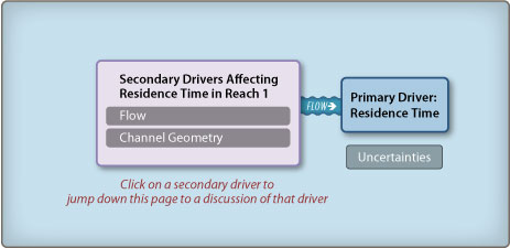
Reach 1: Primary Driver—Residence Time
Residence time is affected by the two secondary drivers shown above. Click on a secondary driver to jump down to the discussion of that driver. See the Basic Concepts page for a general discussion of how the secondary drivers affect the primary driver. Residence time controls the time for algae to grow and BOD to decay in Reach 1. Table 1 indicates that residence time in Reach 1 was 60 hours at a flow of 75 cfs and reduced to 30 hours at a flow of 7,000 cfs. Flow in Reach 1 is primarily governed by the flows contributed to the reach from Friant Dam, tributaries, and other sources (i.e., groundwater discharge) and by agricultural diversions along Reach 1. The figure below shows the measured daily flows along Reach 1; at Newman, located downstream of the Merced River; at Maze, located downstream of the Tuolumne River; and at Vernalis, located downstream of the Stanislaus River. Three eastside tributaries, the Merced, Tuolumne and Stanislaus Rivers, contribute 6580% of the measured flow at Vernalis (Foe et al. 2002).
Table 2 (below) shows the seasonal pattern of Vernalis flows. The average monthly flows are greater than 5,000 cfs from January through May. The median flows are between 2,400 and 3,200 cfs for these same months. The median flow is about 2,000 cfs from June through December. San Joaquin River flows at Vernalis during JuneNovember are much less variable than during the rest of the year (Kratzer et al. 2004).
Throughout most of the year, the San Joaquin River gains water between the mouth of the Merced River and Vernalis; groundwater inputs account for approximately 5% of the total flow in the San Joaquin River (Quinn and Tulloch 2002). Upstream of the Merced River/San Joaquin River confluence, the San Joaquin River may lose water to the adjacent shallow aquifer (Quinn and Tulloch 2002). Irrigation return flows, which can enter the San Joaquin River either via surface water returns or groundwater accretions (i.e., tile drainage), are another source of flows to the San Joaquin River and can account for as much as 13% of the Reach 1 San Joaquin River flows (Quinn and Tulloch 2002). Irrigation diversions from the San Joaquin River in JuneAugust have a significant effect on Reach 1 flows, especially from Crows Landing to Maze Road (Kratzer et al. 2004). At times, upstream agricultural users divert up to 2550% (1,000 to 2,000 cfs) of the San Joaquin River flow at Vernalis (Lee and Jones-Lee 2003). Jump to "Residence Time > Secondary Driver—Flow" under:
Reach 2 |
Reach 3 Secondary Driver—Channel Geometry The San Joaquin River flows in a natural channel through much of Reach 1. Channel geometry is therefore a function of natural riverine processes in this reach. There are levees along most of the channel, but they are far enough away from the low-flow channel to allow some meander of the channel. Table 1 shows the average hydraulic geometry for the San Joaquin River as it relates to the surface area and travel time for a range of flows. The lowest flow in the geometry table is 750 cfs, which was the lowest Vernalis flow during the 1987-1992 drought period. The highest flow shown in the table is 7,000 cfs, which is the highest specified flow during the VAMP period; higher flows are possible during major runoff events with reservoir spills. Table 1 gives the San Joaquin River hydraulic geometry for a range of flows, as determined by the DSM2 hydraulic modeling. Constant flows of 750 to 7,000 cfs along the entire river were simulated with the model to determine the geometry parameters at each flow. Based on stream geometry data from the DSM2-SJR model, the total volume in Reach 1 between the Merced River and Vernalis is 3,761 af at a flow of 750 cfs and 18,229 af at a flow of 7,000 cfs. Because the length is constant, the increase in volume is proportional to the increase in cross-sectional area (i.e., conveyance). The simulated average velocity in Reach 1 increases from 1.4 ft/sec at 750 cfs to 2.4 ft/sec at 7,000 cfs. The corresponding travel time in Reach 1 decreases from 60 hours at 750 cfs to 31 hours at 7,000 cfs. The average surface width in Reach 1 is about 180 feet at 750 cfs and about 400 feet at 7,000 cfs. The corresponding surface area for algae growth, reaeration, and SOD is 1,086 acres at 750 cfs and increases to 2,406 acres at 7,000 cfs. The maximum depth is about 6 feet at 750 cfs and almost 15 feet at 7,000 cfs. The mean depth increases from about 3.5 feet at 750 cfs to about 7.5 feet at 7,000 cfs. Actual flows in Reach 1 will generally be increased substantially by inflows from the Tuolumne and Stanislaus Rivers. However, the Tuolumne and Stanislaus Rivers enter near the downstream end of Reach 1 and increase the flows in this downstream 10-mile portion. The flow below the Merced River (i.e., at Newman) is therefore the best indicator of the travel time and other geometry parameters in Reach 1. Jump to "Residence Time > Secondary Driver—Channel Geometry" under:
Reach 2 |
Reach 3 Uncertainties in Residence Time Residence times and changes in other hydraulic geometry parameters in Reach 1 are well understood through hydraulic modeling and confirmed with dye tracer studies (Kratzer and Biagtan 1997). No major uncertainties were identified in the literature. Although residence time is known to affect algal growth, information is lacking on the direct relationship between increased residence time and increased algal growth (and therefore additional BOD inputs) during periods of low flow. Jump to "Residence Time > Uncertainties in Residence Time" under:
Reach 2 |
Reach 3 |